pslp-lab/file.org

Experiment 1

Objective

Installation of Scilab and demonstration of simple programming concepts like matrix multiplication (scalar and vector), loop, conditional statements and plotting.

Method

1. Installed Scilab binary on desktop via nix package manager.
2. Launched the binary and opened console.

3. Declared matrix and integer, evaluated the product of matrix with a scalar

   Code

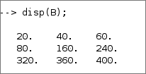
   A = [4 8 12; 16 32 48; 64 72 80];
   x = 5;
   B = x * A;
   disp(B);

   Output

   

4. Declared another matrix and evaluated the vector product

   Code

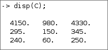
   A = [12 32 54; 9 4 2; 1 2 3];
   B = [1 2 3; 7 2 4; 11 2 13];
   x = 5;
   C= x * A * B;
   disp(C);

   Output

   

5. Declared another matrix and evaluated the dot product

   Code

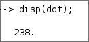
   A = [12 32 54];
   B = [1 2 3];
   dot = A * B';
   disp(dot);

   Output

   

6. Declared another matrix and evaluated the dot product

   Code

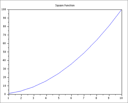
   x = 1:10; 
   y = x .^ 2; 
   plot(x,y); 
   title(‘Square Function’);

   Output

   

Result

Installed Scilab and demonstrated simple programming concepts like matrix multiplication (scalar and vector), loop, conditional statements and plotting.

Experiment-2

Objective

Program for demonstration of theoretical probability limits.

Method

1. Opened Scilab console and evaluated the following commands.
2. Declared integer n and set it to 10000, similarly declared and set another integer head_count to 0.
3. Set up a loop from 1 to 10000 and generated a random number between 0 and 1 using rand() command
4. if the value of number is less then 0.5 then incremented head_count by 1
5. Set up a function P(i) for probability of heads in trial.
6. Plotted the graph of P(i) using plot() command.

Code

n = 10000;
head_count = 0;
for i = 1:n
x = rand(1)

if x<0.5 then
  head_count = head_count + 1;
end

p(i) = head_count / i;
end

disp(p(10000))

plot(1:n,p)
xlabel("No of trials");
ylabel("Probability");
title("Probability of getting Heads");

Output

Result

Experiment 3

Objective

Program to plot normal distributions and exponential distributions for various parametric values.

a) Method: Normal Distribution

1. Opened Scilab console and evaluated the following commands.
2. Declared 2 arrays, m_values and s_values with various parametric values of mean and standard deviation.
3. Set up a loop from 1 to length of the array ‘means’ and got a pair of values of mean and standard deviation.
4. Using those values, generated the probability density function

$f(\boldsymbol{x}) = \frac{1}{s}\cdot\sqrt{2\pi}\cdot e^{\frac{-(\boldsymbol{x} - m) ^ 2}{(2 * s ^ 2)}}$

1. Created a range of x values to plot the normal distribution using linspace() command.
2. Correctly titled and labelled the graph.
3. Plotted various normal distribution curves using plot() command.

a) Code

m_values = [0, 1, -1];
s_values =[0.5, 1, 1.5];

for m = m_values
for s =s_values
  t =grand(1, 1000, "nor", m, s);

  x= linspace(m-4*s, m+4*s, 1000)
  y = (1/s*sqrt(2*%pi))*exp(-(x - m).^2/(2*s^2));

  plot(x, y);
  hold on;
  xgrid();
end

end
legend("m=0, s=0.5", "m=1, s=0.5", "m=-1, s=0.5",...
     "m=0, s=1"  , "m=1, s=1"  , "m=-1, s=1", ...
     "m=0, s=1.5", "m=1, s=1.5", "m=-1, s=1.5");

xlabel("x")
ylabel("Probability density function");
title("Normal distributions for various parametric values");

a) Output

b) Method: Exponential Distribution

1. Opened Scilab console and evaluated the following commands.
2. Declared an array, Lambda_values with various values of lambda
3. Set up a loop from 1 to length of the array Lambda_values and the function grand() is used to generate 1000 random numbers from the exponential distribution.
4. Using those values, generated the probability density function

$f(x) = Y = lambda \cdot e^{-lambda \cdot x}$

1. Created a range of x values to plot the exponential distribution using linspace() command.
2. Correctly titled and labelled the graph.
3. Plotted various exponential distribution curves using plot() command.

b) Code

lambda_values = [0.5, 1, 2];
for lambda = lambda_values
t = grand(1, 1000, "exp", lambda);
x = linspace(0, 8/lambda, 1000);
y = lambda * exp(-lambda * x);

plot(x, y);

xgrid();

hold on;
end

xlabel("x");
ylabel("Probability density function");
title("Exponential distributions for various values of lambda");

legend(["lambda=0.5", "lambda=1", "lambda=2"]);

b) Output

Experiment 4

Objective

Program to plot normal distributions and exponential distributions for various parametric values.

Theory

Binomial Distribution: A probability distribution that summarizes the likelihood that a variable will take one of two independent values under a given set of parameters. The distribution is obtained by performing a number of Bernoulli trials. A Bernoulli trial is assumed to meet each of these criteria:

1. There must be only 2 possible outcomes.
2. Each outcome has a fixed probability of occurring. A success has the probability of p, and a failure has the probability of 1 – p.
3. Each trial is completely independent of all others.
4. To calculate the binomial distribution values, we can use the binomial distribution formula:

$P(X = x) = {}^{n}C_{x} \cdot p^x \cdot (1 - p)^{n - x}$

where `n` is the total number of trials, `p` is the probability of success, and `x` is the number of successes. We can calculate the binomial distribution values for each possible value of `x` using this formula and the values of `n` and `p` given above.

Problem statement

6 fair dice are tossed 1458 times. Getting a 2 or a 3 is counted as success. Fit a binomial distribution and calculate expected frequencies.

Method

1. Find the number of cases, times the experiment is repeated, and the probability of success.
2. Here, we have to find the Binomial Probability Distribution, which is defined as:

$P(X = x) = \frac{n!}{x! \cdot (n-x)!} \cdot s^x \cdot (1 - s)^{n - x}$

Calculate it.

1. Calculate the frequency, which is given by E= P*N.
2. Put the calculated values in the table below.

x	Expected Frequency	Binomial Distribution P (X = x)
0	28.43	0.004831
1	181.83	0.003107
2	547.50	0.009387
3	1009.53	0.017307
4	1213.50	0.020803
5	947.25	0.016255
6	312.50	0.002132

Steps

1. Find the number of cases, here, we take it as n.
2. Find the probability of success. Here, we take it as s (=2/6).
3. Define the number of times the process is repeated, and mark it as N. Here, acc to question, it’s 1458.
4. Take a variable x that varies from 0 to number of cases.
5. Apply the Formula for Binomial Probability Distribution.
6. Apply the formula for the Frequency.
7. Plot the Graph.

Code

n=6;
s=1/3;
N=1458;
x=0:n;
P= (1-s).^(n-x).*s.^x.*factorial(n)./(factorial(x).*factorial(n-x));
E= P*N;
clf();
plot(x,E,"b.-");

Output