17 KiB
Experiment 1
Objective
Installation of Scilab and demonstration of simple programming concepts like matrix multiplication (scalar and vector), loop, conditional statements and plotting.
Method
- Installed Scilab binary on desktop via nix package manager.
- Launched the binary and opened console.
-
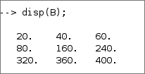
Declared matrix and integer, evaluated the product of matrix with a scalar
Code
A = [4 8 12; 16 32 48; 64 72 80];
x = 5;
B = x * A;
disp(B);
Output
-
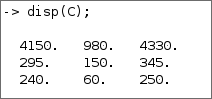
Declared another matrix and evaluated the vector product
Code
A = [12 32 54; 9 4 2; 1 2 3];
B = [1 2 3; 7 2 4; 11 2 13];
x = 5;
C= x * A * B;
disp(C);
Output
-
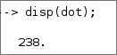
Declared another matrix and evaluated the dot product
Code
A = [12 32 54];
B = [1 2 3];
dot = A * B';
disp(dot);
Output
-
Declared another matrix and evaluated the dot product
Code
x = 1:10;
y = x .^ 2;
plot(x,y);
title(‘Square Function’);
Output
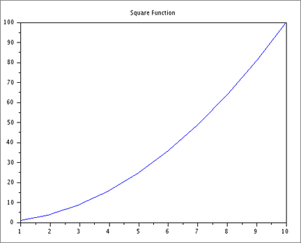


Result
Installed Scilab and demonstrated simple programming concepts like matrix multiplication (scalar and vector), loop, conditional statements and plotting.
Experiment 2
Objective
Program for demonstration of theoretical probability limits.
Method
- Opened Scilab console and evaluated the following commands.
- Declared integer $n$ and set it to 10000, similarly declared and set another integer $head\_count$ to 0.
- Set up a loop from 1 to 10000 and generated a random number between 0 and 1 using rand() command
- if the value of number is less then 0.5 then incremented $head\_count$ by 1
- Set up a function $P(i)$ for probability of heads in trial.
- Plotted the graph of $P(i)$ using plot() command.
Code
n = 10000;
head_count = 0;
for i = 1:n
x = rand(1)

if x<0.5 then
  head_count = head_count + 1;
end

p(i) = head_count / i;
end

disp(p(10000))

plot(1:n,p)
xlabel("No of trials");
ylabel("Probability");
title("Probability of getting Heads");
Output

Result
We see that as the number of lips increase the theoretical probability of 0.5 is approached and the theoretical and practical probabilities become the same.
Experiment 3
Objective
Program to plot normal distributions and exponential distributions for various parametric values.
a) Method: Normal Distribution
- Opened Scilab console and evaluated the following commands.
- Declared 2 arrays, $m\_values$ and $s\_values$ with various parametric values of mean and standard deviation.
- Set up a loop from 1 to length of the array $means$ and got a pair of values of mean and standard deviation.
- Using those values, generated the probability density function
$f(\boldsymbol{x}) = \frac{1}{s}\cdot\sqrt{2\pi}\cdot e^{\frac{-(\boldsymbol{x} - m) ^ 2}{(2 * s ^ 2)}}$
- Created a range of $x$ values to plot the normal distribution using linspace() command.
- Correctly titled and labelled the graph.
- Plotted various normal distribution curves using plot() command.
a) Code
m_values = [0, 1, -1];
s_values =[0.5, 1, 1.5];

for m = m_values
for s =s_values
  t =grand(1, 1000, "nor", m, s);

  x= linspace(m-4*s, m+4*s, 1000)
  y = (1/s*sqrt(2*%pi))*exp(-(x - m).^2/(2*s^2));

  plot(x, y);
  hold on;
  xgrid();
end

end
legend("m=0, s=0.5", "m=1, s=0.5", "m=-1, s=0.5",...
      "m=0, s=1"  , "m=1, s=1"  , "m=-1, s=1", ...
      "m=0, s=1.5", "m=1, s=1.5", "m=-1, s=1.5");

xlabel("x")
ylabel("Probability density function");
title("Normal distributions for various parametric values");
a) Output

b) Method: Exponential Distribution
- Opened Scilab console and evaluated the following commands.
- Declared an array, $lambda\_values$ with various values of $lambda$
- Set up a loop from 1 to length of the array $lambda\_values$ and the function grand() is used to generate 1000 random numbers from the exponential distribution.
- Using those values, generated the probability density function
$f(x) = Y = lambda \cdot e^{-lambda \cdot x}$
- Created a range of $x$ values to plot the exponential distribution using linspace() command.
- Correctly titled and labelled the graph.
- Plotted various exponential distribution curves using plot() command.
b) Code
lambda_values = [0.5, 1, 2];
for lambda = lambda_values
t = grand(1, 1000, "exp", lambda);
x = linspace(0, 8/lambda, 1000);
y = lambda * exp(-lambda * x);

plot(x, y);

xgrid();

hold on;
end

xlabel("x");
ylabel("Probability density function");
title("Exponential distributions for various values of lambda");

legend(["lambda=0.5", "lambda=1", "lambda=2"]);
b) Output

Experiment 4
Objective
Program to plot normal distributions and exponential distributions for various parametric values.
Theory
Binomial Distribution: A probability distribution that summarizes the likelihood that a variable will take one of two independent values under a given set of parameters. The distribution is obtained by performing a number of Bernoulli trials. A Bernoulli trial is assumed to meet each of these criteria:
- There must be only 2 possible outcomes.
- Each outcome has a fixed probability of occurring. A success has the probability of $p$, and a failure has the probability of $1 – p$.
- Each trial is completely independent of all others.
- To calculate the binomial distribution values, we can use the binomial distribution formula:
$P(X = x) = {}^{n}C_{x} \cdot p^x \cdot (1 - p)^{n - x}$
where $n$ is the total number of trials, $p$ is the probability of success, and $x$ is the number of successes. We can calculate the binomial distribution values for each possible value of $x$ using this formula and the values of $n$ and $p$ given above.
Problem statement
6 fair dice are tossed 1458 times. Getting a 2 or a 3 is counted as success. Fit a binomial distribution and calculate expected frequencies.
Method
- Find the number of cases, times the experiment is repeated, and the probability of success.
- Here, we have to find the Binomial Probability Distribution, which is defined as:
$P(X = x) = \frac{n!}{x! \cdot (n-x)!} \cdot s^x \cdot (1 - s)^{n - x}$
Calculate it.
- Calculate the frequency, which is given by E= P*N.
- Put the calculated values in the table below.
| x | Expected Frequency | Binomial Distribution P (X = x) |
|---|---|---|
| 0 | 28.43 | 0.004831 |
| 1 | 181.83 | 0.003107 |
| 2 | 547.50 | 0.009387 |
| 3 | 1009.53 | 0.017307 |
| 4 | 1213.50 | 0.020803 |
| 5 | 947.25 | 0.016255 |
| 6 | 312.50 | 0.002132 |
Steps
- Find the number of cases, here, we take it as $n$.
- Find the probability of success. Here, we take it as $s =2/6$.
- Define the number of times the process is repeated, and mark it as $N$. Here, acc to question, it’s 1458.
- Take a variable $x$ that varies from 0 to number of cases.
- Apply the Formula for Binomial Probability Distribution.
- Apply the formula for the Frequency.
- Plot the Graph.
Code
n=6;
s=1/3;
N=1458;
x=0:n;
P= (1-s).^(n-x).*s.^x.*factorial(n)./(factorial(x).*factorial(n-x));
E= P*N;
clf();
plot(x,E,"b.-");
Output

Experiment 5
Objective
Program for fitting of binomial distributions after computing mean and variance.
Theory
Binomial Distribution: A probability distribution that summarizes the likelihood that a variable will take one of two independent values under a given set of parameters. The distribution is obtained by performing a number of Bernoulli trials. A Bernoulli trial is assumed to meet each of these criteria:
- There must be only 2 possible outcomes.
- Each outcome has a fixed pobability of occurring. A success has the probability of $p$, and a failure has the probability of $1 – p$.
- Each trial is completely independent of all others.
- To calculate the binomial distribution values, we can use the binomial distribution formula:
$P(X = x) = {}^{n}C_{x} \cdot p^x \cdot (1 - p)^{n - x}$
where $n$ is the total number of trials, $p$ is the probability of success, and $x$ is the number of successes. We can calculate the binomial distribution values for each possible value of $x$ using this formula and the values of $n$ and $p$ given above.
Problem statement
A set of three similar coins are tossed 100 ($N$) times with the following results
| No. of Heads ($x$) | 0 | 1 | 2 | 3 |
| Frequency ($f$) | 36 | 40 | 22 | 2 |
Fit a binomial distribution and calculate expected frequencies.
Method
- For given data, total number of coins($n$) = 3 and total number of trials($N$) would be = 100
- Find $X \cdot F$ to calculate the mean, for all corresponding values of $X$ and $F$, and calculate $\Sigma F \cdot x$
Mean would then be = $\frac{\Sigma F \cdot x}{n}$ i.e., $\frac{90}{100} = 0.9$.
- Since we know for binomial distribution, $mean = n \cdot p$. So, $0.9 = 3 \cdot p$ => $p = 0.3$.
- Calculate variance. We already know that $var = n \cdot p \cdot (1-p)$.
- Now, calculate Binomial distribution, $P(X= x)$ and calculate expectes valued using $P \cdot N$.
| $X$ | $F$ | $X \cdot F$ | |
|---|---|---|---|
| / | < | < | <> |
| 0 | 36 | 0 | |
| 1 | 40 | 40 | |
| 2 | 22 | 44 | |
| 3 | 2 | 6 | |
| TOTAL($N$) | 100 | 90 |
| $X$ | 0 | 1 | 2 | 3 | TOTAL |
|---|---|---|---|---|---|
| Observed Frequency | 26 | 40 | 2 2 | 2 | 100 |
| Expected Frequency | 343 | 44.1 | 18.9 | 2.7 | 100 |
Code
n = 3;
N = 100;
F = [36, 40, 22, 2];
X = [0,1,2,3];

FX = (36*0+40*1+22*2+2*3);
Mean = FX/N;
disp("Mean = ", Mean);

p = Mean/n;
disp("Probability of success = ",p);

var = n*p*(1-p);
disp("Variance = ",var);

x = 0:3;
P= (1-p).^(n-x).*p.^x.*((factorial(n))./((factorial(x).*factorial(n-x))));
disp("Binomial distribution = ",P);

E = N*P;
disp("Expected Frequency = ", E);

clf();
plot(X,E,"b.-");

xlabel('X ');
ylabel('Expected Frequency');
title('Binomial Distribution ');

Y = grand(1, 80, "bin", 3,p);
disp(Y);

histplot(30, Y, normalization=%f, style=5);
Output

#+LATEX:\clearpage
Experiment 6
Objective
Program for fitting of Poisson distributions for given value of lambda..
Theory
Poisson Distribution: The Poisson distribution is a discrete probability distribution that expresses the probability of a given number of events occurring in a fixed interval of time or space, assuming that these events occur with a known constant rate and independently of the time since the last event. It is often used to model rare events.
The Poisson distribution has only one parameter, often denoted as $\lambda$, which represents the average rate of occurrence of the events over the given interval. The probability of observing exactly k events in the interval is given by the Poisson probability mass function:
$P(X=k) = (e^{-\lambda} * \lambda^k) / k!$
where $X$ is the random variable representing the number of events, $e$ is the base of the natural logarithm, and $k!$ denotes the factorial of $k$.
The mean and variance of the Poisson distribution are both equal to $\lambda$, which means that the distribution is unimodal and symmetric around $\lambda$.
The Poisson distribution is also a limiting case of the binomial distribution, when the number of trials $n$ goes to infinity and the probability of success $p$ goes to zero, but the product $n \cdot p$ remains constant and equal to $\lambda$.
Problem statement
A set of three similar coins are tossed 100 ($N$) times with the following results in Table 1. Note the difference with experiment number 4 where “observed frequencies” were not given.
| / | < | |||
| No. of Heads ($x$) | 0 | 1 | 2 | 3 |
| Frequency ($f$) | 36 | 40 | 22 | 2 |
Fit a binomial distribution and calculate expected frequencies.
Method
- For given data, create a table (Table 2) to record the values of $x$, $f$, and $xf$. Here, $x$ denotes the number of heads obtained in a single toss, $f$ is the frequency of obtaining $x$ heads, and $xf$ is the product of $x$ and $f$.
| / | < | |||
| $x$ | 0 | 1 | 2 | 3 |
| $f$ | 36 | 40 | 22 | 2 |
| $xf$ | 0 | 40 | 44 | 6 |
- The mean of the binomial distribution can be calculated as $N \cdot p$, where $N$ is the total number of trials and $p$ is the probability of getting a head. Here, $N=100$.
- Calculate the value of $p$, using the formula $p = \frac{x}{N}$, where $x$ is the number of heads obtained in the 100 tosses. So, $p = (036 + 140 + 222 + 32)/100 = 0.64$.
- Using the formula for the binomial distribution, calculate the expected frequency of obtaining x heads in a single toss as:
$P(X = x) = {}^{n}C_{x} \cdot p^x \cdot (1 - p)^{n - x}$
Where $n$ is the total number of trials, $x$ is the number of successful trials, and ${}^{n}C_{x}$ is the binomial coefficient. We can then multiply this value by 100 to get the expected frequency for each value of $x$.
Tabulate this information in Table 3.
| / | < | ||||
| $X$ | 0 | 1 | 2 | 3 | Total |
| Observed Frequency | 36 | 40 | 22 | 2 | 100 |
| Expected Frequency $100 \cdot P(X=x)$ | 23.65 | 37.84 | 27.51 | 10.00 | 100.00 |
Code
observed_freq = [36, 40, 22, 2];
N = sum(observed_freq);
x = 0:3;

mean = sum(x .* observed_freq) / N;

// Poisson distribution with lambda = mean
expected_freq = N * exp(-mean) * (mean .^ x) ./ factorial(x);

// Output tables
disp(["x", "Observed Freq", "Expected Freq"]);
disp([x', observed_freq', expected_freq']);

// Plot of expected frequencies
clf();
plot(x, expected_freq, '.-', 'LineWidth', 2);
xlabel('Number of Heads');
ylabel('Expected Frequency');
title('Fitting of Poisson distribution');
legend('Expected Frequencies');
Output

Experiment 7
Objective:
Plotting Regression line for the given data points.
Formulation and Method
Regression line
where, $m$ = slope, $b$ = y-intercept.
Method of least squares:
Find $\frac{\partial e}{\partial m}, \frac{\partial e}{\partial b} = 0$
Problem statement
Find the regression line for the given data points (x,y)
| X | Y |
|---|---|
| 20 | 0.18 |
| 60 | 0.37 |
| 100 | 0.35 |
| 140 | 0.70 |
| 160 | 0.56 |
| 220 | 0.75 |
| 260 | 0.18 |
| 300 | 0.36 |
| 340 | 1.17 |
| 380 | 1.65 |
Method
- Make $x$ data and $y$ data lists.
- Use regline() to find $m$ and $b$
- Use scatter() to plot $x$ data and $y$ data
- Use plot() to draw regression line.
Results
The following are required as output:
- The full code.
- The plot for regression line and data points.
Code
x_data = [20,60,100,140,160,220,260,300,340,380]
y_data = [0.18,0.37,0.35,0.70,0.56,0.75,0.18,0.36,1.17,1.65]

[a, b] = reglin(x_data, y_data);
scatter(x_data,y_data,30,"x")
plot(x_data, a*x_data+b,"red")

xlabel("X")
ylabel("Y")
title("Simple Linear Regression")
Output
